Technology & Innovation

The Technology and Innovation Committee was created to help promote awareness and increase knowledge for LEMAC membership and industry associates. Through providing this awareness and increasing knowledge sharing, we hope to maximize the use of current and future technologies to improve efficiencies, streamline processes, and develop educational opportunities and resources.

Articles & Presentations

Evaluating a Land System – Questions to Consider 

Data Quality: The Song That Never Ends

Secure Passwords You Can Actually Remember!

LEMAC Data Integrity Reports Final

Adding Data - How do I separate data into multiple columns?

In Excel 2016, “Flash Fill” lets you quickly separate multiple words in a list of cells that are separated by a space; for example, a list of first and last names. Insert a column to the right of the first and last name column. Type in the first or last name of the name in the cell directly to the left and click Enter to take you to the empty cell below. In the Home tab in the Editing section click “Fill” then choose “Flash Fill” or you can do the same thing by going to the Data tab and clicking “Flash Fill” in the Data Tools section. Conversely, you can create a column to join words from multiple columns using the same technique.Accordion Sample Description

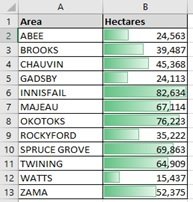
Data Bars - How do I add data bars to my spreadsheet?

Do you want to communicate your numbers visually in Excel?  Data Bars can help. Select your data range, then go to Home > Conditional Formatting > Data Bars, and select a color scheme.

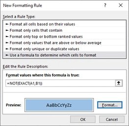
Data Validation - How do I identify differences between columns in Excel?

If you need to quickly identify differences between 2 different columns in Excel, use Conditional Formatting along with a rule. Example, highlight the 2 columns you want to compare. Choose Home > Conditional Formatting and select New Rule. Click on “Use a formula to determine which cells to format” and enter the following formula: =NOT(EXACT(A2,B2)) and then select the Format you want and click OK. (this formula example assumes you want to compare columns A & B starting at row 2 – revise the formula for the columns and rows you want to compare).

Data Validation - How do I set up validation rules in my spreadsheet?
In order to retain the validity of data, sometimes you need to restrict the input value and offer some tips for further steps. For example, to keep well uwis standard to 16 characters, highlight your Well UWI column, go to Data > Data Validation > Settings. Under Allow: select ‘Text length’, under Data: select ‘equal to’, under Length: enter ’16’. Go to the Input Message tab, check the Show input message when cell is selected box, enter a Title such as Well Uwi, and in the Input message box enter “Input a complete 16 character uwi with no slashes or dashes”.
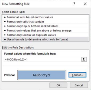
Formatting - How do I shade alternate rows in my spreadsheet?

Option 1: Format as a Table To quickly shade alternate rows, in the Home tab under Styles click on Format as Table, then select the style you prefer and click OK. If you don’t want your data continued to be formatted as a table, click on any field within in your data, in the Table Design tab click on Convert to Range and click Yes. The shading will be maintained until you add additional rows. Option 2: Use a Conditional Formatting Rule Select the entire area you want to apply the rule to. Choose Conditional Formatting > New Rule. In the Select a Rule Type section choose Use a formula to determine which cells to format. In the Edit the Rule Description section enter this formula: =MOD(Row(),2)=1. Click the Format button, move to the Fill tab and choose the color for the shaded rows. Click Ok, Ok. Note: To apply the same rule to Columns rather than rows just change Row to Column in the above formula.

Formatting - How do I auto-fit my column width to my data?

Can’t see all your data in Excel? Just highlight the columns that are too small. Then, under the Home menu, choose Format > AutoFit Column Width.

Formatting - How do I auto-fit my column width to my data?

To auto-fit all your columns at once, click on the arrow at the top left of your spreadsheet to highlight all of your columns, then position your curser right on one of the column separation lines and double-click.

Formattting - How do I hide the columns and rows I don't want to print or show?
To avoid printing specific rows or columns, just hide them before printing. To hide rows, select them by clicking the row numbers (click and drag to select a block of rows; hold down Ctrl while clicking to select non-adjacent rows). Then right-click one of the highlighted border row numbers and click Hide. Use the same procedure to hide columns (but right-click a highlighted column letter to choose Hide).
Formatting - How do I identify duplicate values?
In Excel, do you need to know if there are duplicate values in a column or row? Or maybe the values are intended to be all the same and you need to find out if one is different? Simply select the entire column or row or just a specific range. On the “Home” tab choose “Conditional Formatting > Highlight Cells Rules > Duplicate Values…”. Select either “Duplicate” or “Unique” in the box on the left and from the drop-down list on the right select a color/format and click OK. To remove the formatting highlight the column or range again, choose “Conditional Formatting > Clear Rules > Clear Rules from Selected Cells”
Formatting - How do I quickly highlight all of the data in a worksheet?
Click in cell A1. Press the Control + Shift + End keys simultaneously to highlight all of the data in your worksheet.
Formatting - How do I switch from columns to rows?
Excel “Transpose” copy/paste feature: Have you ever wanted to switch your Excel worksheet columns to rows? Highlight the columns or rows you want to switch, right-click and choose Copy or click the Copy button on the Home tab; move your cursor to the field where you want to paste the data; right-click and under the Paste options choose Transpose (T).
Formatting - How do you apply a change to your entire spreadsheet?
Just click the cell in the top-left corner to select everything. Then apply your change.
Formatting - How do you apply a change to your entire spreadsheet?
Just click the cell in the top-left corner to select everything. Then apply your change.
Formatting - How to change cells to all have the same format?
In Excel, copy the formatting (attributes) of one or more cells and apply them to another cell or range using the Format Painter tool (which looks like a little yellow paintbrush on the Standard toolbar). To format a cell (or cells), select a cell (or cells) that are formatted the way you like and click Format Painter. Then, click and drag to apply that formatting to another cell (or range of cells). This shortcut saves time because you don’t have to manually reapply the font and other attributes to other cells. Alternatively, when pasting one or more cells into another cell range using simply copy-paste, use the CTRL drop down tool along the bottom right after the initial paste action is prompted, and select from a range of pasting options to paste only values, cell formatting, formulas, formulas and number formatting, to keep destination formatting, and more.
Formulas - How do I add the current date and time to a cell?
Here is how to insert the current date or time in an Excel spreadsheet, which will update itself every time you open the file. Enter “=NOW()” into any cell. (Excel will display the date and time formatted according to the regional options you’ve set for Windows.) If you just want to see the date, use the today function: “=TODAY()”
Formulas - How do I copy a formula down in my spreadsheet?
Select the cell with the formula that you want to copy down; hover your curser over the little square box in the lower right hand corner of the cell until the cursor turns into a cross-hair; then double click.
Formulas - How do I add the current date and time to cell and prevent it from changing?
To insert a fixed date into a cell (a date that you don’t want to change) hold down Ctrl while you press the semicolon (;) key. To insert the current time (without a date), press Ctrl-Shift-;
Formulas - How do I merge or concatenate the contents of cells together?
In Excel, let’s say you have text values in cells A1 thru C1 and you want cell D1 to be all three of those values combined. Just use this simple formula in cell D1: =A1&B1&C1.
Formulas - How do I quickly remove slashes and dashes from a UWI?

To remove slashes and dashes from a UWI in Excel, apply the following formula: =(SUBSTITUTE(SUBSTITUTE(A1,”/”,””),”-“,””))

Keyboard Shortcuts - How do I create a new workbook using my keyboard?
Press the Ctrl key + the N key simultaneously while you have the Excel application open.
Keyboard Shortcuts - How do I insert rows or columns using the keyboard?
Press Alt-I, then C to insert a column – new columns will be inserted to the left of your current column. Press Alt-I, then R to insert a row – new rows will be inserted above your current column.
Keyboard Shortcuts - How do I select an entire column or row in my spreadsheet using my keyboard?
Navigate to a cell in the row or column you want to select and hold down the Shift + Space Bar for the row or the Control + Space Bar for the column.
Searching - How do I add subtotals quickly?
To quickly add subtotals to a list in Excel, first sort the document by the column you want subtotals for by clicking on the “Data” tab. Move your cursor to one of the cells within your list and click “Sort” in the “Sort & Filter” group. In the “Sort” window select which column you want to sort by and click “OK”. Then click on “Subtotal” in the “Outline” group. In the “At each change in” dialog box select the column you want to subtotal by. In the “Use function” dialog box select the type of subtotal you want (i.e. Sum, Count, Average). In the “Add subtotal to” dialog box select the column you want the subtotals to appear in. Check the “Summary below data” box and click OK.

Systems & Website Links

Government/Regulator Web-based Programs, Information, and Available Data – June 2018